Freeze Multiple Rows in Excel

Freezing Multiple Rows in Excel: A Step-by-Step Guide

When working with large datasets in Excel, it can be challenging to keep track of headers or important information as you scroll through the spreadsheet. One solution to this problem is to freeze multiple rows in Excel, allowing you to lock specific rows in place while still being able to scroll through the rest of your data. In this article, we will explore how to freeze multiple rows in Excel, including the benefits and potential drawbacks of this technique.

Benefits of Freezing Multiple Rows

Freezing multiple rows in Excel can be incredibly useful for several reasons: * Improved readability: By keeping headers or important information visible at all times, you can more easily understand the context of your data. * Enhanced navigation: Freezing rows can help you quickly identify specific sections of your spreadsheet, making it easier to navigate large datasets. * Increased productivity: With important information always in view, you can work more efficiently and reduce the need to constantly scroll back to the top of your spreadsheet.

How to Freeze Multiple Rows in Excel

Freezing multiple rows in Excel is a relatively straightforward process. Here are the steps to follow: * Select the row below the rows you want to freeze. For example, if you want to freeze the first two rows, select the third row. * Go to the “View” tab in the ribbon and click on “Freeze Panes.” * Select “Freeze Panes” and then choose “Freeze Panes” again from the dropdown menu. * Alternatively, you can also use the keyboard shortcut “Alt + W + F” to freeze panes.

📝 Note: Make sure to select the row below the rows you want to freeze, as this will determine which rows are locked in place.

Freezing Multiple Rows Using the Freeze Panes Option

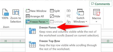
Another way to freeze multiple rows is by using the “Freeze Panes” option. Here’s how: * Select the cell below the rows you want to freeze. * Go to the “View” tab and click on “Freeze Panes.” * Select “Freeze Panes” and then choose “Freeze Top Row” or “Freeze First Column” depending on your needs. * If you want to freeze multiple rows, select the row below the rows you want to freeze and then use the “Freeze Panes” option.

Unfreezing Rows in Excel

If you need to unfreeze rows in Excel, you can do so by following these steps: * Go to the “View” tab in the ribbon and click on “Freeze Panes.” * Select “Unfreeze Panes” from the dropdown menu. * Alternatively, you can also use the keyboard shortcut “Alt + W + F” to unfreeze panes.

Tips and Tricks for Freezing Rows

Here are some additional tips and tricks to keep in mind when freezing rows in Excel: * Use multiple freeze points: You can freeze multiple rows and columns in Excel by selecting different cells and using the “Freeze Panes” option. * Use the split screen feature: Excel also allows you to split the screen into multiple panes, which can be useful for comparing data or working on different parts of a spreadsheet. * Experiment with different freeze points: Don’t be afraid to experiment with different freeze points to find the one that works best for your specific needs.

Freeze Option	Description
Freeze Top Row	Freezes the top row of the spreadsheet
Freeze First Column	Freezes the first column of the spreadsheet
Freeze Panes	Freezes the selected row or column
Unfreeze Panes	Unfreezes the selected row or column

In terms of common issues, some users may experience problems with frozen rows not staying in place or with the “Freeze Panes” option not working as expected. To troubleshoot these issues, try restarting Excel or checking for any conflicts with other add-ins or plugins.

Best Practices for Freezing Rows

Here are some best practices to keep in mind when freezing rows in Excel: * Keep it simple: Avoid freezing too many rows or columns, as this can make it difficult to navigate your spreadsheet. * Use clear headers: Use clear and descriptive headers to help you quickly identify the frozen rows. * Experiment with different layouts: Don’t be afraid to experiment with different layouts and freeze points to find the one that works best for your specific needs.

In conclusion, freezing multiple rows in Excel can be a powerful tool for improving readability, navigation, and productivity. By following the steps outlined in this article and using the tips and tricks provided, you can unlock the full potential of freezing rows in Excel and take your spreadsheet skills to the next level. Whether you’re working with large datasets or simply need to keep important information visible, freezing rows is a technique that can help you achieve your goals.